Analysis¶

The Analysis class is the primary class which will provide methods for analyzing your life data. This class is designed to take your data and calculate \(\beta\) and \(\eta\) values along with generating any appropriate plots for display of your data.

A typical use case of the Analysis case is as follows:

import weibull

# fail times include no censored data
fail_times = [
    9402.7,
    6082.4,
    13367.2,
    10644.6,
    8632.0,
    3043.4,
    12860.2,
    1034.5,
    2550.9,
    3637.1
]

# this is where the actual analysis and curve fitting occur
analysis = weibull.Analysis(fail_times, unit='hour')

Fitting¶

The fit() method is used to calculate appropriate \(\beta\) and \(\eta\) values, which are then stored into the class instance. When fit() is called with no parameters, then the linear regression method of calculation is assumed:

analysis.fit()

An alternative method is to use the Maximum Likelihood Estimation (MLE) method of fitting \(\beta\) and \(\eta\) to the data. This may be done by specifying that the method='mle':

analysis.fit(method='mle')

In many cases, the mle and lr methods will yield very similar values for \(\beta\) and \(\eta\), but there are some cases in which one is preferred over the other. It turns out that linear regression tends to work best for very low sample sizes, usually less than 15 while the maximum likelihood estimator works best for high sample sizes. In both cases, the probplot() method should be used to verify that the data is a good fit.

To retrieve the \(\beta\) and \(\eta\) values, simply use the instance variables beta and eta:

print(f'beta: {analysis.beta: .02f}')
print(f'eta: {analysis.eta: .02f}')

When using the fit() method, it is also possible to set the confidence levels

Use the stats() method to get a pandas.Series containing most internal estimates:

$> analysis.stats
fit method          maximum likelihood estimation
confidence                                    0.6
beta lower limit                          2.42828
beta nominal                              2.97444
beta upper limit                          3.64344
eta lower limit                           186.483
eta nominal                               203.295
eta upper limit                           221.622
mean life                                  181.47
median life                               179.727
b10 life                                   95.401
dtype: object

Plotting¶

One of the most often requested features of such a package is plotting the data, particularly in Jupyter Notebooks. The weibull package comes with built-in methods to easily display and save standard plots with one-line methods.

Building on the analysis instance above, we will examine the probability plot:

analysis.probplot()

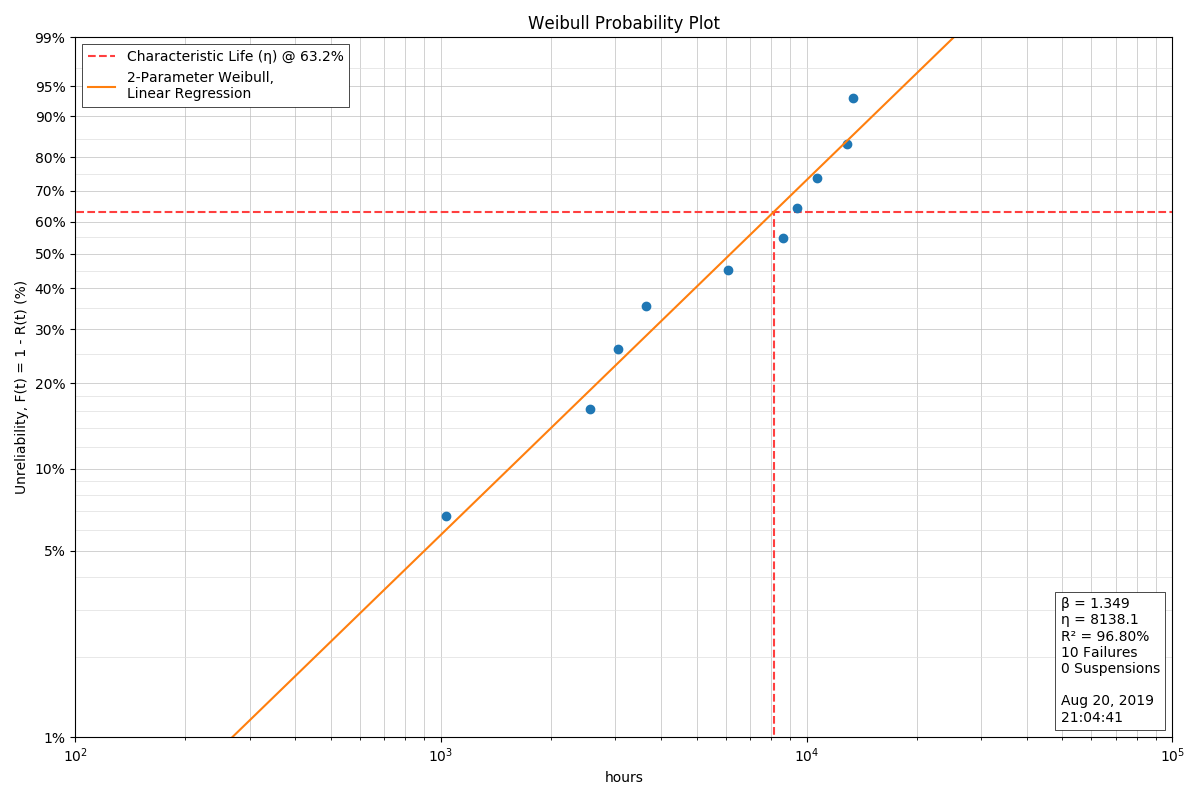
There are some settings for the Weibull probability plots that will allow the user to add more information to the plot itself that are useful when the plot will be included in reports, on web pages, or other situations where the supporting information may not always accompany the plot. These include being able to specify the Analyst’s name and/or the Company or Organization name:

analysis.analyst = 'John Q. Smith'
analysis.company = 'Smith & Smith Engineering'

It should be noted that if either the Analyst or Company name is especially long, the annotation box (where they are displayed) will expand to fit the text which could obscure some portions of the Weibull plot. To address this, you can place a line feed '\n' within either name which will force the text to wrap to a shorter length. These must be defined before calling the probplot function.

Also, the user can now provide their own more descriptive title for the plot, use the default title, or suppress the title altogether, as follows:

analysis.plot_title = 'Weibull Analysis of Golden Widget Failures'

Setting the title to a zero-length string (or not defining one at all) will cause the default title of ‘Weibull Probability Plot’ to be used. Setting the title to None will suppress the title line altogether. Any other value set for analysis.plot_title will be displayed on the Weibull plot. This too must be defined before calling the probplot function.

By default, the probability plot will now be 12 inch x 8 inch (1200 x 800 pixels) to better display enhancements made to the plot format, but it is also possible to change the size of the plot to a different size or aspect ratio by specifying the figsize:

plt.figure(figsize=(8, 6))
analysis.probplot()

where the values of 8 and 6 are in inches (at 100px/inch). Be aware that generating plots smaller than the default size may result in the Y-Axis labels overlapping one another (especially when analyzing very large data sets), or the annotation box might covering some portion of the Weibull plot or the Characteristic Life line. You may have to experiment with the size values to get a satisfactory result, and you may also need to use the image resizing features when inserting the image into a document or presentation.

We can also examine a number of other common function plots (only the hazard plot is shown, but the others are along the same line):

analysis.pdf()
analysis.sf()
analysis.hazard()
analysis.cdf()

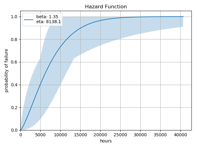
Each of these functions will generate a plot that is suitable for publication or insertion into a Jupyter Notebook. Again, note that some of these methods - such as hazard() and cdf() will produce the same plot with slightly different labeling.

Confidence Levels¶

Some plots will contain a shaded region which reflects the confidence_levels. The confidence levels are calculate for \(\beta\) and \(\eta\) and the min/max values for \(\beta\) and \(\eta\) are explored rather than all possible values. As a result, the visualizations shown are an approximation of the confidence limits.

Class Documentation¶

class weibull.Analysis(data: list, suspended: list = None, unit: str = 'cycle')¶

Calculates and plots data points and curves for a standard 2-parameter Weibull for analyzing life data.

Parameters:

data – A list or numpy array of life data, i.e. [127, 234, 329, 444]
suspended – A list or numpy array of suspensions as boolean values, i.e. [False, False, True, True]. At any point which indicates True means that the test was stopped - or that the item was removed from the test - before the item failed.
unit – The unit (‘hour’, ‘minute’, ‘cycle’, etc.). This is used to add some useful information to the visualizations. For instance, if the unit is hour, then the x-axis will be labed in hours.

Variables:

beta – The current value of the shape parameter, \(\beta\). This value is initially set to None. The proper value for beta will be calculated on call to the fit() method. The user may also set this value directly.
eta – The current value of the scale parameter, \(\eta\). This value is initially set to None. The proper value for beta will be calculated on call to the fit() method. The user may also set this value directly.
_fit_test – Basic statistics regarding the results of fit(), such as \(R^2\) and P-value.

b(percent_failed: (<class 'float'>, <class 'str'>) = 10.0)¶

Calculate the B-life value

Parameters:	percent_failed – the number of elements that have failed as a percent (i.e. 10)
Returns:	the life in cycles/hours/etc.

cdf(show: bool = True, file_name: str = None, watermark_text=None)¶

Plot the cumulative distribution function

Parameters:	show – True if the plot is to be shown, false if otherwise file_name – the file name to be passed to `matplotlib.pyplot.savefig` watermark_text – the text to include as a watermark
Returns:	None

characteristic_life¶

Returns the current characteristic life of the product, aka \(\eta\)

Returns:	the characteristic life of the product

failures¶

Returns the number of failures in the data set.

Returns:	the number of failures in the data set

fit(method: str = 'lr', confidence_level: float = 0.9)¶

Calculate \(\beta\) and \(\eta\) using a linear regression or using the maximum likelihood method, depending on the ‘method’ value.

Parameters:	method – ‘lr’ for linear estimation or ‘mle’ for maximum likelihood estimation confidence_level – A number between 0.001 and 0.999 which expresses the confidence levels desired. This confidence level is reflected in all subsequent actions, especially in plots, and can also affect several internal variables which are shown in `stats`.
Returns:	None

fr(show: bool = True, file_name: str = None, watermark_text=None)¶

Plot failure rate as a function of cycles

Parameters:	show – True if the item is to be shown now, False if other elements to be added later file_name – if file_name is stated, then the probplot will be saved as a PNG watermark_text – the text to include as a watermark
Returns:	None

hazard(show: bool = True, file_name: str = None, watermark_text=None)¶

Plot the hazard (CDF) function

Parameters:	show – True if the plot is to be shown, false if otherwise file_name – the file name to be passed to `matplotlib.pyplot.savefig` watermark_text – the text to include as a watermark
Returns:	None

mean¶

Calculates and returns mean life (aka, the MTTF) is the integral of the reliability function between 0 and inf,

\[MTTF = \eta \Gamma(\frac{1}{\beta} + 1)\]

where gamma function, \(\Gamma\), is evaluated at \(\frac{1}{\beta+1}\)

Returns:	the mean life of the product

median¶

Calculates and returns median life of the product

Returns:	The median life

mttf¶

Calculates and returns mean time between failures (MTTF)

Returns:	the mean time to failure

pdf(show: bool = True, file_name: str = None, watermark_text=None)¶

Plot the probability density function

Parameters:	show – True if the plot is to be shown, false if otherwise file_name – the file name to be passed to `matplotlib.pyplot.savefig` watermark_text – the text to include as a watermark
Returns:	None

probplot(show: bool = True, file_name: str = None, watermark_text=None, **kwargs)¶

Generate a probability plot. Use this to show the data points plotted with the beta and eta values.

Parameters:	show – True if the plot is to be shown, false if otherwise file_name – the file name to be passed to `matplotlib.pyplot.savefig` watermark_text – the text to include on the plot as a watermark kwargs – valid matplotlib options
Returns:	None

r_squared¶

Returns the r squared value of the fit test

Returns:	the r squared value

sf(show: bool = True, file_name: str = None, watermark_text=None)¶

Plot the survival function

Parameters:	show – True if the plot is to be shown, false if otherwise file_name – the file name to be passed to `matplotlib.pyplot.savefig` watermark_text – the text to include as a watermark
Returns:	None

stats¶: Returns the fit statistics, confidence limits, etc :return: a pandas series containing the fit statistics

suspensions¶

Returns the number of suspensions in the data set.

Returns:	the number of suspensions in the data set

Analysis¶

Fitting¶

Plotting¶

Confidence Levels¶

Class Documentation¶

Related Topics

Table of Contents